Truncated Wigner method

In this example, we simulate the quantum properties of a coherently driven polariton fluid using the truncated Wigner method. In particular, we will compute the steady-state momentum distribution and the second-order correlation function in momentum space, g₂(k, k'). This will teach us how to include noise terms in our simulations, and how to extract quantum statistical properties from the results. We will see the appearance of strong correlations between modes with opposite momenta, which are a signature of pair production processes in the fluid.

Theoretical Background

The truncated Wigner method is a powerful technique for simulating the quantum dynamics of many-body systems. It approximates the quantum field by a classical stochastic field with appropriate initial conditions and noise terms. The stochastic differential equation we solve in this method takes the form:

\[i d\psi = \left( -\delta - i \frac{\gamma}{2} - \frac{\hbar \nabla^2}{2m} + g (|\psi|^2 - \frac{1}{\text{dx}}) \right)\psi dt + F dt + \sqrt{\frac{\gamma}{2\text{dx}}} dW(x,t)\]

Here, ψ is the polariton field, δ is the detuning, γ is the decay rate, m is the effective mass, g is the nonlinearity strength, F is the coherent pump, and dW(x,t) is a complex Wiener process.

For more details on the derivation and validity of the truncated Wigner method, see [1, 2].

Simulation of the steady state

First, let's simulate the system without noise to establish the steady-state solution. This will serve as our reference point for understanding the quantum effects that appear when we add noise.

using GeneralizedGrossPitaevskii, FFTW, CairoMakie, Statistics

We define the equation components according to our stochastic differential equation above. The dispersion relation includes the kinetic energy, detuning, and decay terms:

function dispersion(ks, param)
    param.ħ * sum(abs2, ks) / 2param.m - param.δ - im * param.γ / 2
end;

The pump is spatially uniform and constant in time:

function pump(x, param, t)
    param.A
end;

The nonlinearity includes a -1/dx regularization term:

nonlinearity(ψ, param) = param.g * (abs2(first(ψ)) - 1 / param.dx);

Now we define the physical parameters for a typical polariton system:

ħ = 0.6582
γ = 0.047 / ħ
m = 1 / 6
g = 3e-4 / ħ
δ = 0.49 / ħ
A = 10;

Grid and parameters for a 1D system:

L = 512
N = 256
dx = L / N

lengths = (L,)
param = (; ħ, m, δ, γ, g, A, L, dx)

(ħ = 0.6582, m = 0.16666666666666666, δ = 0.7444545730780917, γ = 0.07140686721361288, g = 0.0004557885141294439, A = 10, L = 512, dx = 2.0)

We initialize the field to zero and solve the mean-field Gross-Pitaevskii equation without noise:

u0 = (zeros(ComplexF64, N),);
prob = GrossPitaevskiiProblem(u0, lengths; dispersion, nonlinearity, pump, param)
nsaves = 512
dt = 0.05
tspan = (0, 200)
alg = StrangSplitting()
ts, sol = solve(prob, alg, tspan; nsaves, dt, show_progress=false);

Let's examine how the density at one spatial point evolves toward steady state:

ns = abs2.(sol[1][1, :])

with_theme(theme_latexfonts()) do
    fig = Figure()
    ax = Axis(fig[1, 1]; xlabel="t", ylabel="n")
    lines!(ax, ts, ns; linewidth=2)
    fig
end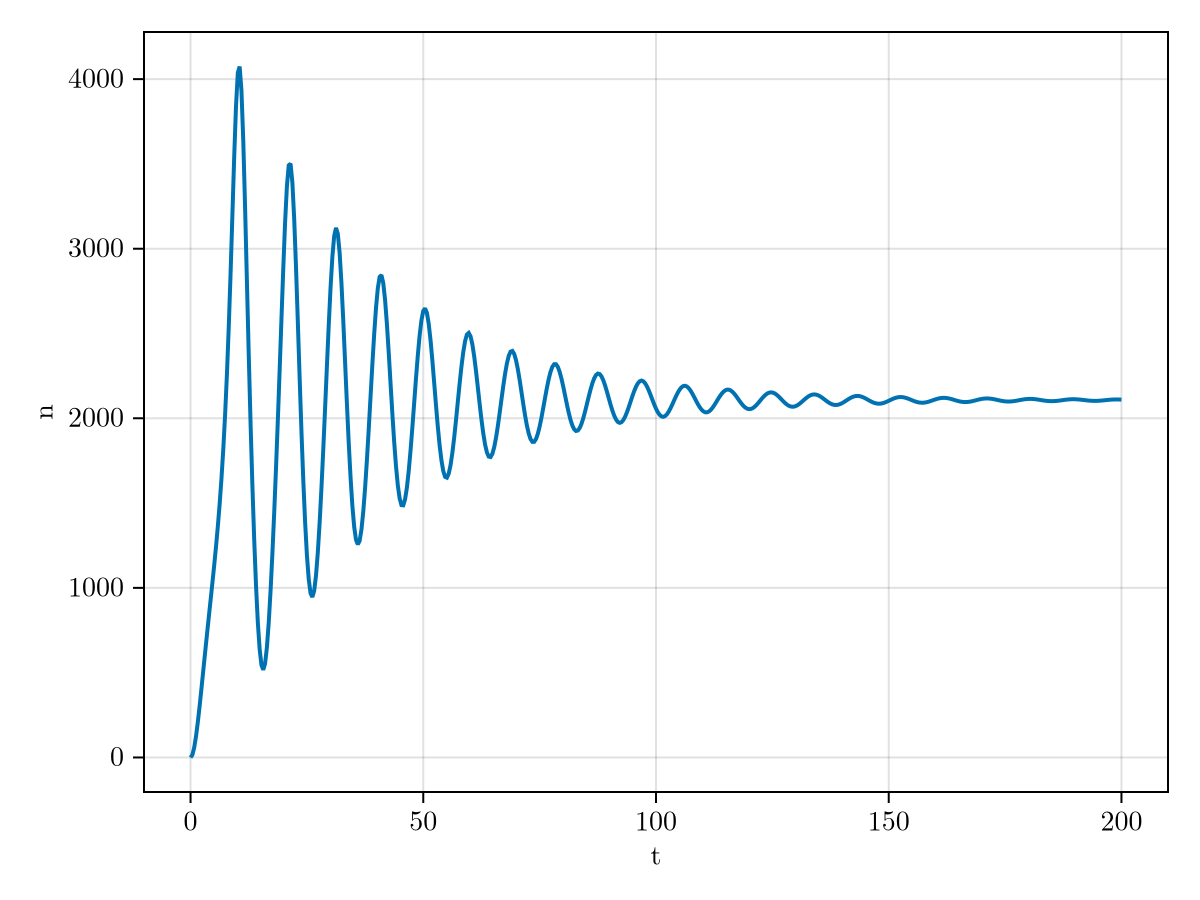

We can see the density approaches a steady-state value, confirming that our system reaches equilibrium.

Inclusion of quantum noise

Now we implement the full truncated Wigner method by including quantum noise. In this approach, we run many stochastic trajectories with random initial conditions and noise terms. Each trajectory represents one possible realization of the field evolution.

We initialize with random Gaussian noise in the field amplitudes, as required by the Wigner representation of the vacuum state. We also define a second dimension that represents the ensemble of stochastic trajectories.

u0 = (randn(ComplexF64, N, 256) / √(2dx),);

The noise prototype specifies the shape and type of the noise to be added at each time step. In this case, it matches the shape and type of the initial condition.

noise_prototype = similar.(u0);

The position noise function corresponds to the √(γ/2dx) dW(x,t) term in our stochastic equation:

position_noise_func(ψ, xs, param) = √(param.γ / (2param.dx));

Now we solve the problem with noise included:

prob = GrossPitaevskiiProblem(u0, lengths; dispersion, nonlinearity, pump, param, noise_prototype, position_noise_func)
ts, sol = solve(prob, alg, tspan; nsaves=1, dt, save_start=false, show_progress=false);

Extraction of quantum statistical properties

From the ensemble of stochastic trajectories, we can extract quantum statistical properties that are not accessible in classical mean-field simulations.

Occupation number in momentum space

First, we transform to momentum space and calculate the average occupation number:

ft_sol = fftshift(fft(sol[1], 1), 1) / N
ks = fftshift(fftfreq(N, 2π / dx));

The momentum distribution n(k) is obtained by averaging |ψ(k)|² over all trajectories, with a correction term of -1/(2L) to account for the Wigner representation:

nks = dropdims(mean(abs2, ft_sol; dims=2), dims=(2, 3)) .- 1 / (2L)

with_theme(theme_latexfonts()) do
    fig = Figure(; fontsize=16)
    ax2 = Axis(fig[1, 1]; xlabel="k", ylabel="n(k)")
    ylims!(ax2, 0, 0.0025)
    lines!(ax2, ks, nks, linewidth=2)
    fig
end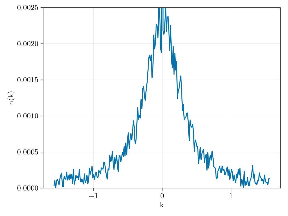

The momentum distribution shows a symmetric peak at k=0 and tails extending to finite momentum. The result is noisy, but this is solved by simply increasing the number of stochastic trajectories.

Second-order correlation function in momentum space

Now we calculate the second-order correlation function g₂(k,k'), which reveals quantum correlations between different momentum modes. This quantity is defined as:

\[g_2(k, k') = \frac{\langle \hat{\psi}_1^*(k) \hat{\psi}_2^*(k') \hat{\psi}_1(k) \hat{\psi}_2(k') \rangle}{n(k) n(k')}\]

where $\hat{\psi}$ denotes quantum field operators.

In the Wigner representation, we must include corrections to account for the symmetrically ordered nature of the representation. Therefore, the calculation of g₂(k,k') from the stochastic fields requires the formula:

\[\langle \hat{\psi}^{\dagger}(k) \hat{\psi}^{\dagger}(k') \hat{\psi}(k') \hat{\psi}(k) \rangle = \left\langle |\psi(k)|^2 |\psi(k')|^2 - \frac{1}{2L}(1 + \delta_{k,k'}) \cdot \left( |\psi(k)|^2 + |\psi(k')|^2 - \frac{1}{2L} \right) \right\rangle_W\]

where ⟨...⟩_W denotes averaging over the stochastic trajectories in the Wigner representation.

We define now some helper functions to compute this quantity correctly:

function f(x, y, δ, commutator)
    abs2(x) * abs2(y) - (1 + δ) * commutator / 2 * (abs2(x) + abs2(y) - commutator / 2)
end

function G2(sol, commutator)
    result = similar(sol, real(eltype(sol)), (size(sol, 1), size(sol, 1)))

    for n ∈ axes(result, 2), m in axes(result, 1)
        result[m, n] = mapreduce((x, y) -> f(x, y, m == n, commutator), +,
            view(sol, m, :), view(sol, n, :)) / size(sol, 2)
    end

    result
end;

Now we calculate the correlation function:

G2k = G2(ft_sol, 1 / L)
g2k = G2k ./ (nks * nks');

Visualize the correlation function:

with_theme(theme_latexfonts()) do
    fig = Figure(; fontsize=16, size=(500, 400))
    ax = Axis(fig[1, 1]; xlabel=L"k", ylabel=L"k'", aspect=DataAspect())
    xlims!(ax, -0.6, 0.6)
    ylims!(ax, -0.6, 0.6)
    hm = heatmap!(ax, ks, ks, g2k, colorrange=(0, 3))
    Colorbar(fig[1, 2], hm, label=L"g_2(k, k')")
    fig
end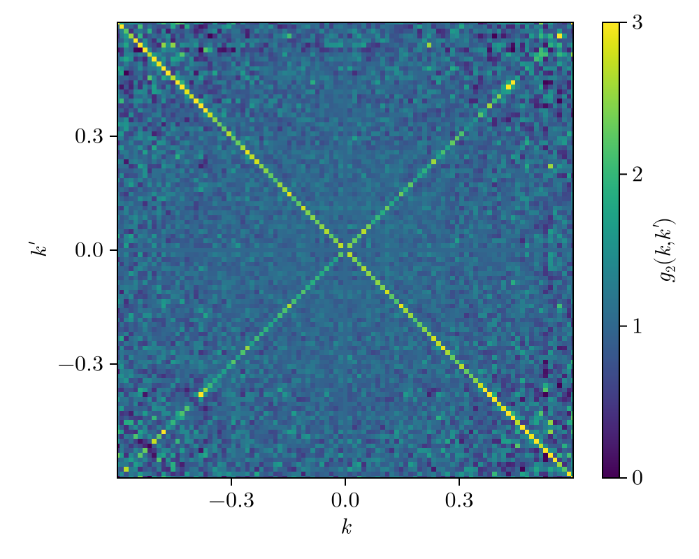

The correlation function reveals strong correlations along the anti-diagonal (k ≈ -k'), which is a signature of spontaneous pair production processes in the driven-dissipative fluid. This quantum effect cannot be captured by classical mean-field theories and demonstrates the power of the truncated Wigner method for studying quantum many-body phenomena.

This page was generated using Literate.jl.