Bistability in the Polariton Condensate

This example demonstrates the bistability phenomenon in a polariton condensate. The mean field equations describing this system may possess two stable solutions for certain parameters. They can be reached by varying the pump intensity, inducing a hysteresis loop. Here, we show the theoretical bistability curve and compare it with the results from a numerical simulation.

First we load the necessary packages:

using GeneralizedGrossPitaevskii, CairoMakie

The analytical solution

The mean field of the polariton condensate is described by a driven dissipative Gross-Pitaevskii equation of the form

\[i \frac{\partial \psi}{\partial t} = F(x, t) + \left( - \delta - i \frac{\gamma}{2} - \frac{\hbar \nabla^2}{2m} + g |\psi|^2 \right)\psi\]

In the above, ψ represents the wave function of the polariton condensate, which is a complex-valued function of space and time, F(x, t) is an external pump, which is a monochromatic term detuned from the cavity resonance by a frequency δ, γ is the decay rate of the polaritons, ħ is the reduced Planck constant, m is the effective mass of the polaritons, and g is the strength of the nonlinear interaction.

Here we define the numerical values of some of the parameters

ħ = 0.654 # (meV*ps)
m = 1 / 3
g = 0.01
δ = 0.3
γ = 0.1;

It can be shown that, in a steady and homogeneous state, the intensity I = |F|^2 necessary to support the fluid at a given density n is given by the following function:

function bistability_curve(n, δ, g, γ)
    n * (γ^2 / 4 + (g * n - δ)^2)
end;

Here, this theoretical curve is displayed:

ns_theo = LinRange(0, 41, 512)
Is_theo = bistability_curve.(ns_theo, δ, g, γ)

with_theme(theme_latexfonts()) do
    fig = Figure(fontsize=16)
    ax = Axis(fig[1, 1]; xlabel="I", ylabel="n")
    lines!(ax, Is_theo, ns_theo, color=:blue, linewidth=4, label="Theoretical")
    fig
end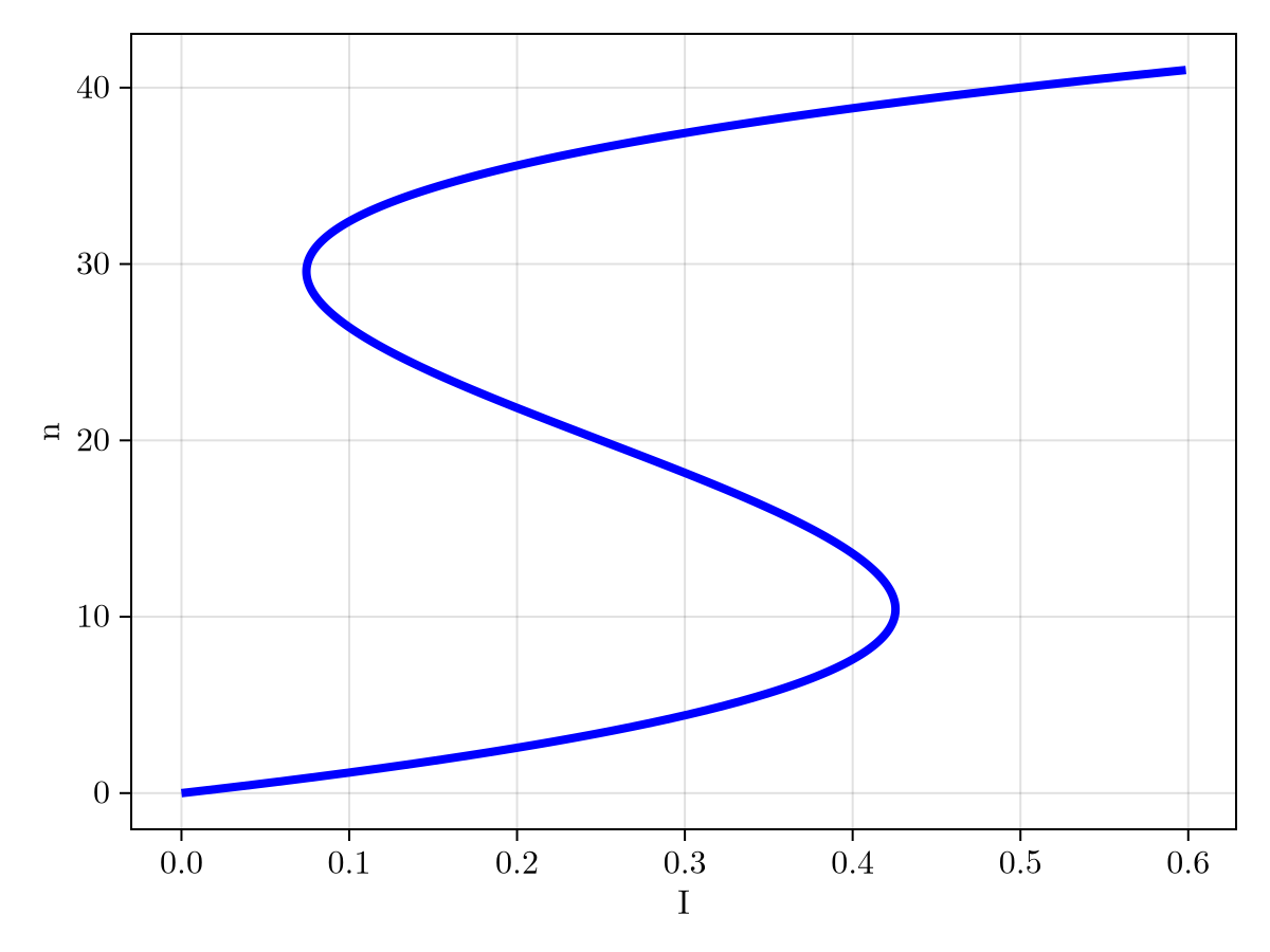

It can be seen that, for certain values of the parameters, the system exhibits bistability, with two stable solutions for the same pump intensity.

The numerical solution

Now, we wish to reproduce the bistability curve using a numerical simulation. This is achieved by slowly varying the pump intensity and observing the resulting steady-state densities. The first step is to specify the equations governing the system.

Here is the dispersion term, which models the Laplacian in Fourier space. As these are constants, we also include the detuning and decay terms.

function dispersion(ks, param)
    param.ħ * sum(abs2, ks) / 2param.m - param.δ - im * param.γ / 2
end;

Next, we define the nonlinear term.

nonlinearity(ψ, param) = param.g * abs2(ψ[1]);

Finally, we define the pump profile. Here, we define the time-dependent pump intensity, which is a parabola that has zeros at t=0 and t=2tmax, and a maximum Imax at t=tmax.

function I(t, tmax, Imax)
    val = -Imax * t * (t - tmax) * 4 / tmax^2
    val < 0 ? zero(val) : val
end;

We also define the complete pump profile, which includes both the spatial and temporal components. The spatial profile is a Gaussian centered in the middle of the system.

function pump(x, param, t)
    exp(-sum(abs2, x .- param.L / 2) / param.width^2) * √I(t, param.tmax, param.Imax)
end;

We now choose the numerical values of the pump constants:

tmax = 4000
Imax = maximum(Is_theo)
width = 50;

We now define the spatial grid used in the simulation:

L = 256
lengths = (L,)
N = 128

128

The initial condition is a vector of zeros, corresponding to an initially empty cavity.

u0 = (zeros(ComplexF64, N),);

Now the time parameters are defined:

dt = 0.1
tspan = (0, tmax);

Also, we define the number of saves and the algorithm to use.

nsaves = 512
alg = StrangSplitting();

Finally, we collect all the necessary parameters in a named tuple

param = (; tmax, Imax, width, δ, ħ, m, γ, g, L);

Now, we define the problem and obtain the solution:

prob = GrossPitaevskiiProblem(u0, lengths; dispersion, nonlinearity, pump, param)
ts, sol = solve(prob, alg, tspan; dt, nsaves, show_progress=false);

In the following plot, we can see the evolution of the density over time.

with_theme(theme_latexfonts()) do
    xs = (0:N-1) * (L / N)
    fig = Figure(fontsize=24)
    ax = Axis(fig[1, 1]; xlabel=L"x", ylabel=L"t")
    heatmap!(ax, xs, ts, abs2.(sol[1]); colormap=:viridis, colorrange=(0, 40))
    fig
end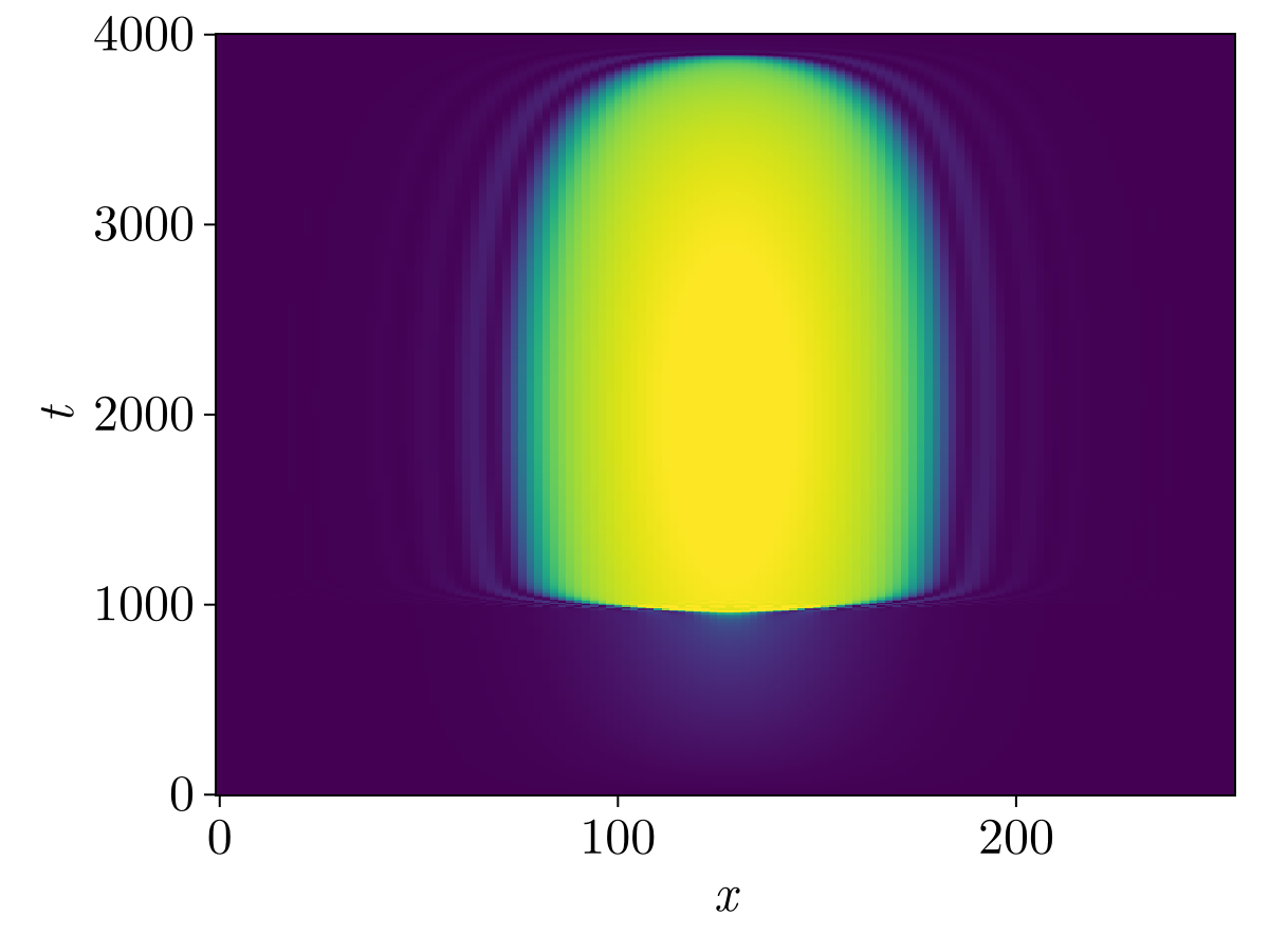

As expected, the density slowly rises as we increase the pump intensity. When the tip of the lower branch is reached, the system jumps suddenly to the upper branch. A backwards behavior is observed when decreasing the pump intensity, where the system can jump back to the lower branch.

Finally, we can compare the simulation results with the theoretical predictions. We do this by plotting the density as a function of the pump intensity.

The pump intensity is given by the function I(t, tmax, Imax) calculated at the saved time points.

Is = I.(ts, tmax, Imax);

On the other hand, the density is obtained from the solution evaluated at the center of the cavity, which is where the pump attains its maximum value.

ns = abs2.(sol[1][N ÷ 2, :]);

Now, we plot the results, comparing with the theory discussed earlier.

with_theme(theme_latexfonts()) do
    fig = Figure(fontsize=24)
    ax = Axis(fig[1, 1]; xlabel="I", ylabel="n")
    lines!(Is, ns; label="Simulation", color=:red, linewidth=5)
    lines!(ax, Is_theo, ns_theo, color=:blue, linewidth=5, label="Theory", linestyle=:dash)
    axislegend(ax, position=:rb)
    fig
end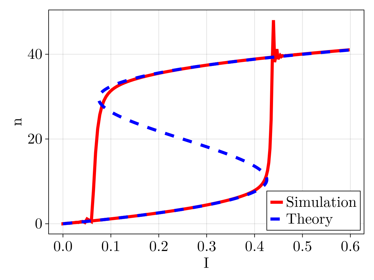

We can see that the simulation closely matches the theoretical predictions,

This page was generated using Literate.jl.